NBA Game Prediction System Using Composite Stacked Machine Learning Model
Abstract
Predicting NBA games is not an easy task. Conventional data analysis and statistic approaches are usually complicated and the accuracy is not high. In this work, a machine learning based method is proposed and the complete design flow is thoroughly introduced and explained. 8 single-stage machine learning models are trained and compared. More complex composite models such as voting mechanism and stacking method are also designed and elaborated. The proposed model reaches 76.8% accuracy on predicting all 2018 NBA playoffs. Furthermore, for the Eastern Conference Final, Western Conference Finals, and Conference Finals, our model achieves an extraordinary prediction accuracy of 85.7%, 71.4%, and 100%, respectively. The source code and dataset are available
here.
Problem Definition
The mission of this work is to precisely predict NBA games' winning and losing result. Machine learning models are trained to predict game results based on the information of two teams' recent status. The idea is expressed as in Figure 1. Beside game-winning prediction, information of the prediction's confidence level is also valuable for us to understand how intense the matchup might be.
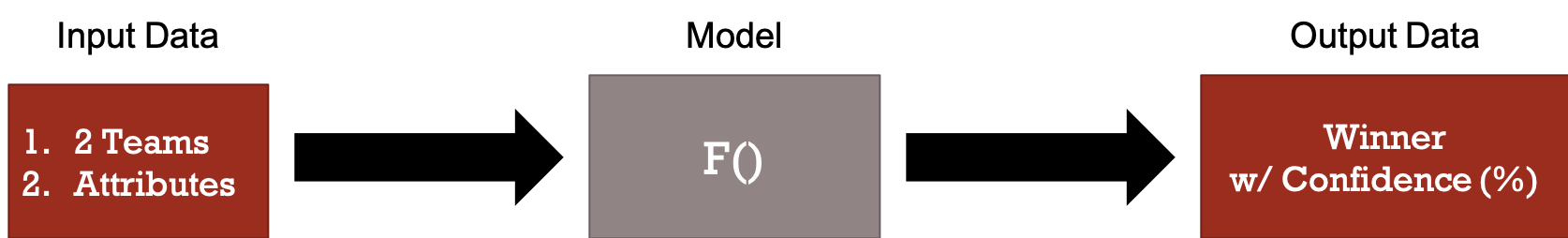
Figure 1: Problem definition.
Dataset
This work predicts NBA games based on the dataset collected from the
official NBA stats website. A crawler program is designed to scrape the game boxes and save the data automatically. Details about the crawler design are available
here. NBA games, including seasons and playoffs, from 1985 to 2018 are collected. The dataset contains 68,458 season matches and 4,816 playoff matches. Figure 2 shows the number of games played by all 30 NBA teams. Due to various history from each team, the number of games for 30 teams are not homogeneous. Moreover, since there are at most 16 teams entitled to enter playoff each year, the number of playoff games played by each team is different as well.
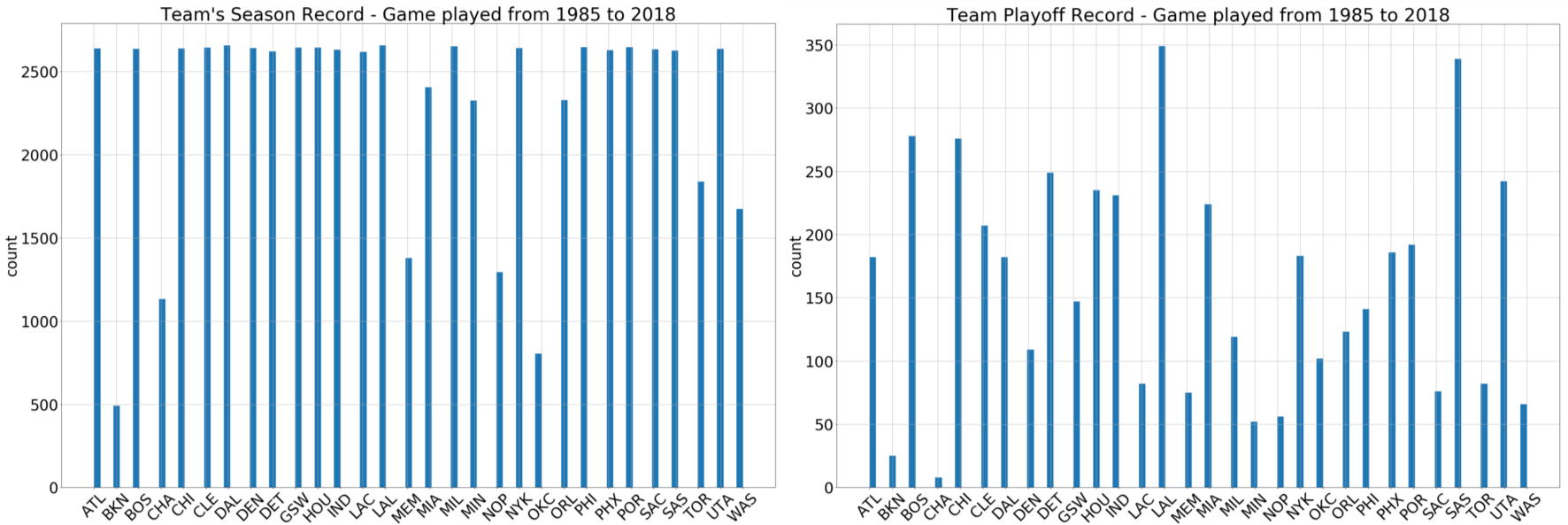
Figure 2: Statistics of the number of games played by each NBA team.
Before processing our data, a classification regarding data types is conducted. Table 1 shows data types of the dataset. As we can see, most of the data are numeric. There is one categorical data, Team, and there are two binary data, Win/Lose and Home/Away. Our target is to precisely predict which team wins a game when two teams meet. Therefore, Win/Lose is the label and our machine learning model predicts the Win/Lose outcome and provides the confidence level of its prediction.
Table 1: Type of Attirbutes
| Binary |
Win/Lose, Home/Away |
| Categorical |
Team |
| Numeric |
Date, PTS, FG%, FGM, FGA, 3P%, 3PM, 3PA, FT%, FTM, FTA, REB, OREB, DREB, AST, STL, BLK, TOV, PF |
Data Preprocessing and Feature Extraction
Typical data preprocessing is conducted as shown in Figure 3. Preprocessing includes data cleaning, one-hot encoding, numeric data normalization, game pairing, validity checking, etc. The final legitimate data volume is 61,368, including seasons and playoffs.
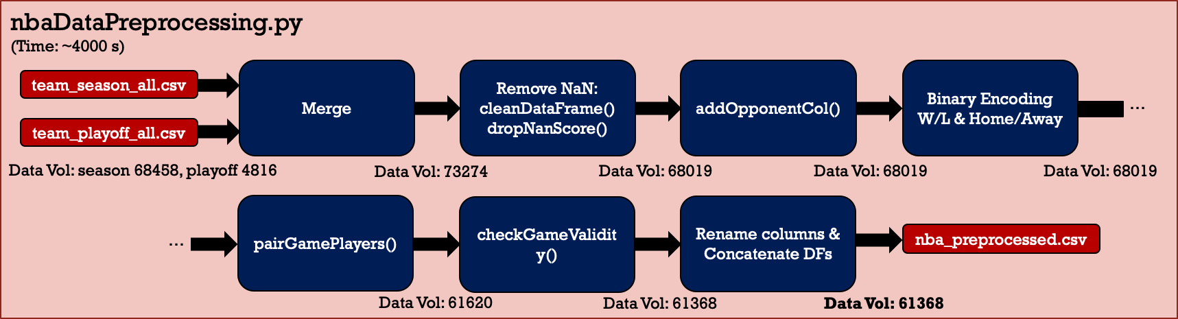
Figure 3: Data preprocessing flow chart.
To train machine learning models, feature extraction is carried out as shown in Figure 4 and 5. Firstly, select the attributes that are more representative to the winning or losing of games. Then, put all selected attributes in a vector. The attribute X is the average performance considered from previous games played by two teams prior to the date we target to predict. In other words, attribute X represents the teams' recent status. Label Y is Win/Lose since we would like to predict which team wins the game.
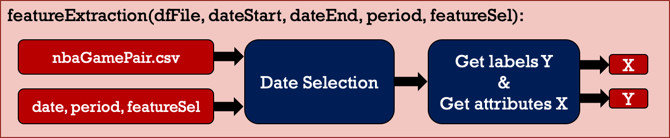
Figure 4: Feature extraction.
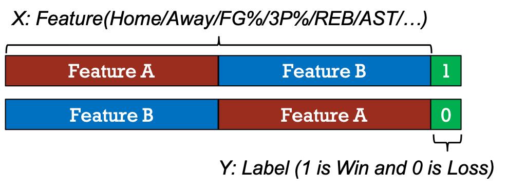
Figure 5: How attribute X and label Y look like.
Model Training and Testing
After data preprocessing and feature extraction are completed, model training and testing can proceed. In this section, grid search with cross validation is firstly applied to find the optimal model parameters. Afterward, data size evaluation is conducted to help us understand how data volume influences the model performance. Then, voting and stacking models are introduced. At last, a comprehensive performance comparison of different machine learning models is presented.
Grid Search with Cross Validation
8 different frequently used single-stage machine learning models are analyzed in this work. Model parameters are optimized by grid search. To prevent possible overfitting issue that happens frequently in model training, cross validation is applied. Table 2 presents which parameters are considered and in what ranges are they examined. Note that since the Naïve Bayes model has no parameters to choose, it does not require grid search.
Table 2: Grid Search Parameters
| Model |
Parameters Sweeping Table |
Model |
Parameters Sweeping Table |
| Logistic Regression | 'C': [0.001, 0.01, 0.1, 1, 10, 100, 1000],
'max_iter': [100, 200, 300, 400, 500] |
GBDT | 'loss': ['deviance', 'exponential'],
'n_estimators': [600, 800, 1000],
'learning_rate': [0.1, 0.2, 0.3],
'max_depth': [3, 5, 10],
'subsample': [0.5],
'max_features': ['auto', 'log2', 'sqrt'] |
| SVM | 'C': [0.01, 0.1, 1, 10, 100],
'kernel': ['rbf', 'linear'],
'gammas': ['auto', 0.001, 0.01],
'shrinking': [True, False] |
LightGBM | 'learning_rate': [0.1, 0.2, 0.3],
'n_estimators': [600, 800, 1000],
'max_depth': [-1, 5, 10],
'subsample' : [0.5] |
| XGBoost | 'max_depth': [3, 5, 7],
'learning_rate': [0.1, 0.3],
'n_estimators': [100, 200, 300],
'min_child_weight': [1, 3],
'gamma': [x/10 for x in range(0, 5)] |
AdaBoost | 'learning_rate': [1, 0.1, 0.2, 0.3],
'n_estimators': [50, 100, 600, 800, 1000] |
| Random Forest | 'n_estimators': [600, 800, 1000],
'criterion': ['gini', 'entropy'],
'bootstrap': [True, False],
'max_depth': [None, 5, 10],
'max_features': ['auto', 'log2', 'sqrt'] |
Naïve Bayes | N/A |
Data Size Evaluation
The data size evaluation is an important step when training models. Since the play style of NBA games changes rapidly as time goes, training models using more data does not mean a better prediction accuracy. As a result, the relation between training data size and performance is evaluated and the outcome is presented in Table 3. As shown in the table, training data covering three-year previous games presents the best performance and it is chosen as the optimal dataset for all our models.
Table 3: Data Size Evaluation
| Training Data (yr) |
Training Data (#) |
Accuracy (%) |
| LogiRegr |
SVM |
XGBoost |
Naïve Bayes |
Random Forest |
GBDT |
LightGBM |
AdaBoost |
| 1 | 2460 | 69.6 | 70.9 | 74.7 | 60.8 | 68.4 | 72.2 | 68.4 | 73.4 |
| 2 | 5078 | 70.9 | 72.2 | 72.2 | 59.5 | 69.6 | 69.6 | 74.7 | 68.4 |
| 3 | 7234 | 70.9 | 74.7 | 74.7 | 60.8 | 70.9 | 73.4 | 68.4 | 76.0 |
| 4 | 9370 | 69.6 | 72.2 | 72.2 | 59.5 | 72.2 | 70.9 | 73.4 | 73.4 |
| 5 | 11702 | 70.9 | 70.9 | 76.0 | 59.5 | 74.7 | 74.7 | 69.6 | 74.7 |
Voting
To prevent bias from a single machine learning model, a voting mechanism, as shown in Figure 6, is applied to make the prediction decision more convincing. 5 machine learning models, including Logistic Regression, SVM, XGBoost, GBDT, and AdaBoost, are considered in the voting model owing to their better performance. The voting mechanism is simple. The decision agreed by most of the models is the final decision. Furthermore, the ratio of agreed votes to total votes is an indicator implying the confidence level of the final decision.
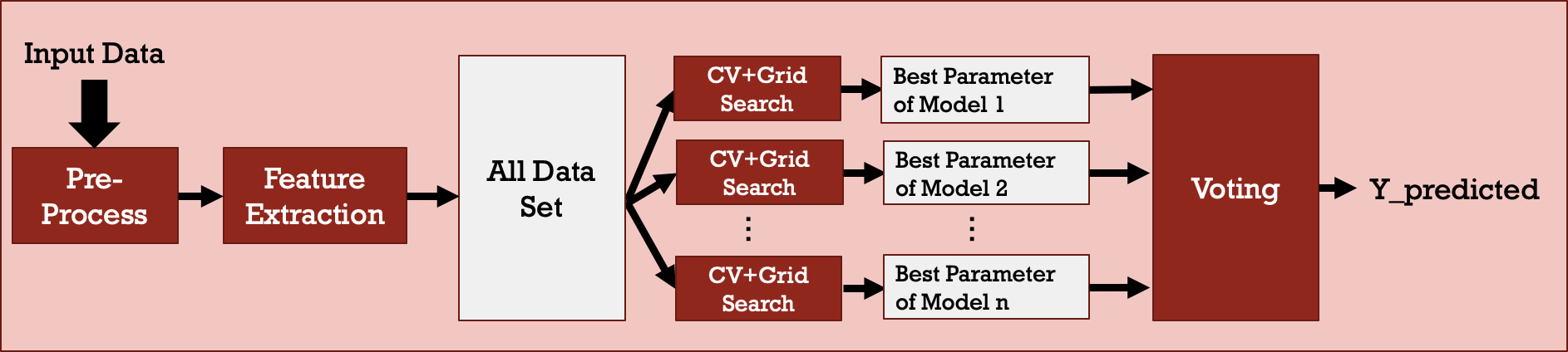
Figure 6: Voting model.
Stacking
Stacking is a more sophisticated approach that consolidates the predictions from multiple well-trained models and uses them as a new set of training attributes to train another model. It can be considered a multi-stage model or a stacked model that is helpful for preventing bias from certain models. At some level, is can be seen as a mode complicated voting mechanism. Figure 7 shows the block diagram of the stacking model and the details of how stacking works are presented in Figure 8. In this work, several combinations of different machine learning models constructing the stacked model are evaluated. In addition, both 2-stage and 3-stage stacked models are analyzed.
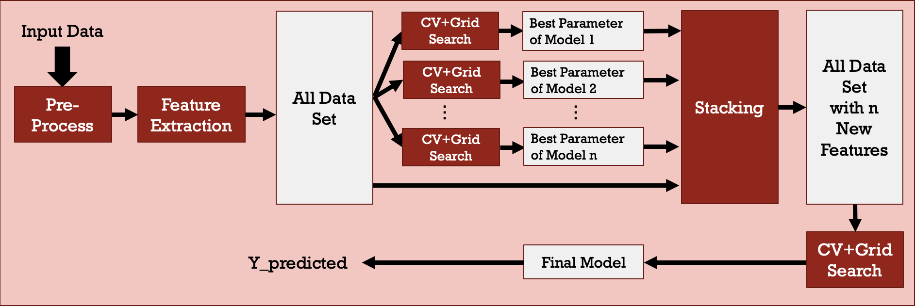
Figure 7: Stacking model.
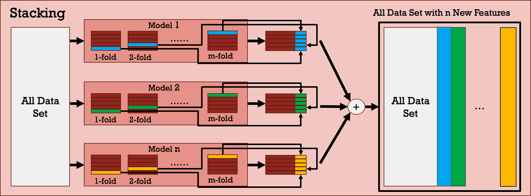
Figure 8: Details in stacking block.
As shown in Table 4, 3-stage stacking model is slightly better than 2-stage stacking model. To thoroughly consider all models, 2-stage stacking of SVM/GBDT/XGBoost + AdaBoost and 3-stage stacking of SVM/XGBoost + RF/GBDT + AdaBoost are selected for the consideration of the final performance comparison.
Table 4: Stacking Model Performance Evaluation
| Stacking |
Stage 1 |
Stage 2 |
Final Stage |
Total Estimators (#) |
Prediction Accuracy (%) |
| 2-Stage |
| SVM/GBDT/XGBoost | None | AdaBoost | 4 | 76.8 (1st) |
| SVM/GBDT/AdaBoost | None | XGBoost | 4 | 74.4 |
| SVM/XGBoost/AdaBoost | None | GBDT | 4 | 72.0 |
| XGBoost/GBDT/AdaBoost | None | SVM | 4 | 73.2 |
| SVM/RF/GBDT/XGBoost | None | AdaBoost | 5 | 74.4 |
| SVM/RF/GBDT/AdaBoost | None | XGBoost | 5 | 72.0 |
| 3-Stage |
| SVM/XGBoost | RF/GBDT | AdaBoost | 5 | 76.8 (1st) |
| RF/GBDT | SVM/XGBoost | AdaBoost | 5 | 75.6 |
| SVM/AdaBoost | RF/GBDT | XGBoost | 5 | 75.6 |
| RF/GBDT | SVM/AdaBoost | XGBoost | 5 | 75.6 |
| SVM/RF | XGBoost/GBDT | AdaBoost | 5 | 75.6 |
Experimental Results
This work evaluates eight single-stage models, one voting model, one 2-stage stacked model, and one 3-stage stacked model. The performance comparison is summarized in Table 5. We can observe that for the single-stage estimators, all models have decent prediction accuracy except for Naïve Bayes and LightGBM. Moreover, composite models such as voting and stacking are even more accurate than single-stage estimators. AdaBoost, 2-stage stacked, and 3-stage stacked models possess the peak performance of 76.8 % prediction accuracy. In conclusion, stacked machine learning model is an appropriate approach for our task.
Table 5: 2018 NBA Playoff Game Winning Prediction
| Model |
Algorithms/Architectures |
Prediction Accuracy (%) |
| Single-Stage Estimator |
| Logistic Regression | 72.0 |
| SVM | 75.6 |
| XGBoost | 75.6 |
| Naïve Bayes | 62.2 |
| Random Forest | 72.0 |
| GBDT | 74.4 |
| LightGBM | 69.5 |
| AdaBoost | 76.8 |
| Voting |
Logistic Regreesion/SVM/XGBoost/GBDT/AdaBoost | 73.2 |
| 2-Stage Stacking |
SVM/GBDT/XGBoost + AdaBoost | 76.8 |
| 3-Stage Stacking |
SVM/XGBoost + RF/GBDT + AdaBoost | 76.8 |
The most important games in the NBA are Eastern/Western Finals and the Conference Finals. GBDT is applied as an example to show our predictions on each game as shown in Table 6. The accuracy of the model prediction manifests the tension of the games to some extent. For example, in the 2018 NBA Conference Finals, Golden State Warriors swept Cleveland Cavaliers and our model precisely predicted the fact without incorrect predictions. As shown in the table, only one game had a confidence level lower than 60% and that game was indeed more intense than the other three games. As for Eastern and Western Conference Finals, since both matchups were more competitive, the resulting confidence level of our model was lower compared to the Conference Finals. In summary, this work designs a machine learning model that can reach prediction accuracy of 85.7%, 71.4%, and 100% for Eastern Conference Final, Western Conference Finals, and Conference Finals, respectively.
Table 6: 2018 NBA Finals/Semi-Finals Game Winning Prediction by GBDT Model
| Game (#) |
Home |
Away |
Actual Winner |
Predicted Winner |
Confidence (%) |
Accuracy (%) |
| NBA Conference Finals |
| 1 |
GSW |
CLE |
GSW |
GSW |
70.9 |
100.0 |
| 2 |
GSW |
CLE |
GSW |
GSW |
68.9 |
| 3 |
CLE |
GSW |
GSW |
GSW |
58.3 |
| 4 |
CLE |
GSW |
GSW |
GSW |
62.3 |
| NBA Western Conference Finals |
| 1 |
HOU |
GSW |
GSW |
GSW |
56.3 |
71.4 |
| 2 |
HOU |
GSW |
HOU |
HOU |
53.9 |
| 3 |
GSW |
HOU |
GSW |
GSW |
50.2 |
| 4 |
GSW |
HOU |
HOU |
GSW |
64.2 |
| 5 |
HOU |
GSW |
HOU |
HOU |
60.0 |
| 6 |
GSW |
HOU |
GSW |
GSW |
54.0 |
| 7 |
HOU |
GSW |
GSW |
HOU |
63.7 |
| NBA Eastern Conference Finals |
| 1 |
BOS |
CLE |
BOS |
BOS |
53.6 |
85.7 |
| 2 |
BOS |
CLE |
BOS |
BOS |
58.9 |
| 3 |
CLE |
BOS |
CLE |
CLE |
61.2 |
| 4 |
CLE |
BOS |
CLE |
CLE |
61.3 |
| 5 |
BOS |
CLE |
BOS |
BOS |
57.8 |
| 6 |
CLE |
BOS |
CLE |
CLE |
55.9 |
| 7 |
BOS |
CLE |
CLE |
BOS |
51.8 |