TrackNet Optimization by Parallel Programming
Abstract
Parallel programming is a powerful methodology that can utilize multicore computation units to accelerate program execution. A highly parallelizable program can reach an exceptional speedup if proper parallelism is adopted. However, if the program is natively non-parallelizable and can only execute in a sequential manner, there is no margin for acceleration with the help of parallel programming. This paper exploits the power of parallelism to speedup TrackNet, a deep learning neural network capable of accurately tracking tiny fast-moving objects. An actual 10-minute badminton competition broadcast video is analyzed. 18,243 frames are processed with parallelism mechanism. For Task I: Frame Retrieval from Video, 6-core multiprocessing achieves 2.73 speedup and the total saved time is 344.59 seconds. For Task II: Generating Heatmaps, 6-core multiprocessing achieves as high as 3.97 speedup and the total saved time is 2227.09 seconds. For Task III: TrackNet Model Evaluation, 6-core multiprocessing achieves 1.47 speedup and the total saved time is 17.22 seconds. With parallel programming, both image pre-processing and post-preprocessing processes are significantly accelerated, making the entire object tracking flow much more efficient than before.
Introduction
TrackNet is a deep neural network capable of tracking fast-moving tiny objects. Developing TrackNet is motivated by information retrieval from sports videos. If enough amount of data is collected, in-depth sports analysis can be conducted and provide meaningful suggestions for coaches and players to improve their performance. TrackNet is firstly applied to tracking badminton trajectory by retrieving coordinates in broadcast videos. TrackNet can be illustrated as Figure 1. To build up a complete database for future analysis, including machine learning and data mining tasks, immense data are expected to be retrieved from a large number of videos. Therefore, retrieving the data from videos in an efficient way is momentous, leading us to the motivation of speeding up TrackNet.

Figure 1: Problem definition of TrackNet.
In order to improve the processing speed of TrackNet, parallel programming is intuitively considered. As shown in Figure 2, the complete TrackNet flow can be divided into three parts: video/image pre-processing, TrackNet model training and predicting, and video/image post-processing. Since TrackNet is trained based on TensorFlow framework which is accelerated by CUDA with NVIDIA GPU, this work does not focus on the model training due to the little margin for speedup. On the other hand, programs of video/image pre-processing and post-processing were written in a sequential manner, possessing immense potential for improvement.
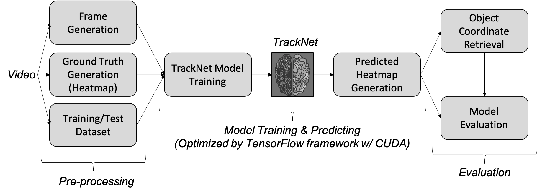
Figure 2: Flow chart of TrackNet.
Before the action of parallelizing the program, the coarse program profiling is performed. Frame generation, heatmap generation, and model evaluation are the three time-consuming blocks and the execution time are 544.16, 2977.31, and 54.07 seconds, respectively. As for training dataset and test dataset generation, since it only involves file arrangement without image processing and actions of saving or loading images, the execution time is less than 1 second. As a result, there is no practical need for improvement. In this paper, the mentioned three programs are to be accelerated by multicore processing and they are listed as below.
- Task I: Frame Retrieval from Video
- Task II: Generating Heatmaps
- Task III: TrackNet Model Evaluation
Proposed Solution
Task I: Frame Retrieval from Video uses VideoCapture() function of OpenCV to retrieve frames from video in a sequential manner. The block diagram of the program is shown in Figure 3. Each frame is cut and retrieved from the complete video so that the next frame can be revealed. Since the retrieval process is completely continuous and indivisible, it cannot be parallelized. However, our task is not only retrieving frames but also saving all frames as jpg files. Parallelism on Task I still worths a try. In fact, the program execution of saving frames takes much longer time than retrieving frames and it is parallelizable.
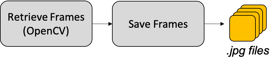
Figure 3: Block diagram of Task I: Frame retrieval from video.
To profile the program of Task I, a test case if a 10 minutes video with a frame rate of 30 FPS is used. There are 18,243 frames to be retrieved and saved as jpg files. In the sequential execution, retrieving frames takes 65.60 seconds and saving frames takes 479.11 seconds. In other words, retrieving frames accounts for 11.95% and saving frames accounts for 88.05%. Since retrieving frames is not parallelizable and saving frames is highly parallelizable, we conclude that the potential parallelizable proportion takes 88.05% of the overall program. As shown in the profiling outcome, the proportion of the non-parallelizable section is not low, so the expected performance of program acceleration is moderate.
The proposed solution to speedup Task I is to parallelize the saving frames function. Since each image is independent of each other, the order does not matter, implying that each core can independently execute the job of saving images. The idea is illustrated as Figure 4. Assuming that there are x frames and n processors, we assign x/n frames to each processor so that the workload is evenly distributed to all processors. During the frame retrieval part, an array used to contain all frames retrieved from the video. When distributing jobs to processors, the array is evenly divided and each processor loads the frames that it is responsible for.
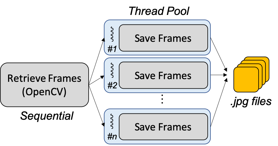
Figure 4: Proposed Parallelism on Task I: Frame retrieval from video.
Task II: Generating Heatmaps imports the badminton coordinate label file, retrieves the coordinates of each frame, generates corresponding heatmaps according to the coordinates, and save these heatmaps. The block diagram of Task II is shown in Figure 5. Except for importing badminton coordinate label file, the other three blocks including getting coordinates, generating heatmaps, and saving heatmaps are expected to be parallelizable in terms of data parallelism. As a result, significant improvement is expected.
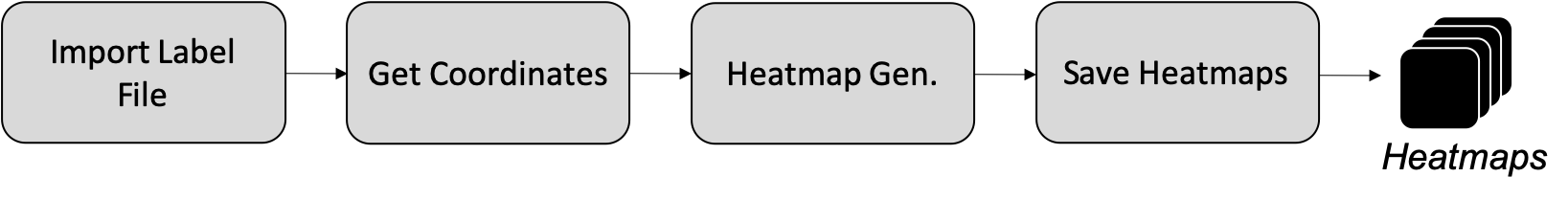
Figure 5: Block diagram of Task II: Generating heatmaps.
The program profiling of Task II is conducted using a test case of generating 18,243 heatmaps. In the sequential execution, importing label file accounts for less than 0.1% of the entire task II. Getting coordinates, generating heatmaps, and saving heatmaps account for larger than 99.9%. Since importing label file is not parallelizable and the other three blocks are all highly parallelizable, we conclude that the potential parallelizable proportion takes 99.9% of the overall program. Hence, an enormous amount of time is expected to be saved when we adopt parallel programming on Task II.
Intuitively, the proposed solution to speedup Task II is to parallelized the mentioned three parallelizable functions. The reason they can be parallelized is that all heatmaps are independent of each other. Hence, a feasible way is to use an array to contain all coordinates of each frame and distribute the workload evenly to all processes to achieve the load balance. Since the output of the program is png files, each processor can directly save complete heatmap as png files without extra communication with other processors. The proposed solution is illustrated as Figure 6.
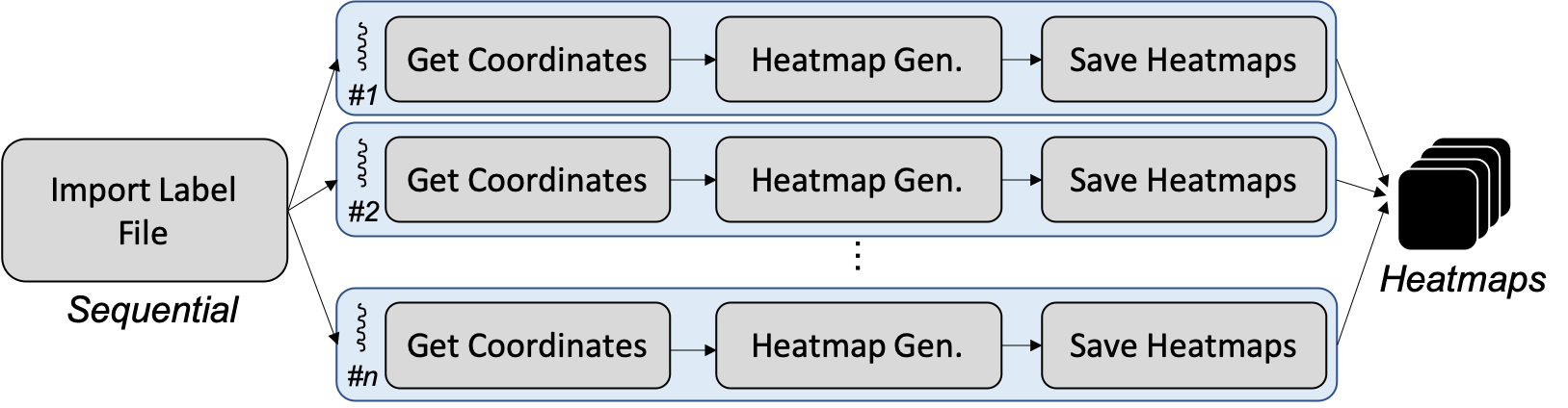
Figure 6: Proposed Parallelism on Task II: Generating heatmaps.
Task III: TrackNet Model Evaluation includes five functions. Importing the randomly selected 30% test dataset from a file, loading corresponding TrackNet model predicted heatmaps, detecting circles by Hough Circles function provided by OpenCV, building confusion matrix, and finally calculating precision and recall to evaluate the predicting performance. The block diagram of Task III is shown in Figure 7. Importing test dataset and calculating precision/recall are two non-parallelizable functions. Fortunately, the execution time of these two non-parallelizable blocks is very short compared with the other parallelizable blocks. As Task II, since the proportional of parallelizable functions dominate in terms of execution time, a promising speedup is expected.

Figure 7: Block diagram of Task III: TrackNet Model Evaluation.
The program profiling of Task III is conducted using the randomly selected test dataset which includes 5,472 frames. In the sequential execution, both importing test dataset from file and calculating precision/recall account for only less than 0.1% of the entire program. The rest of blocks, including loading predicted heatmaps, detecting circles by Hough Circles API, and building confusion matrix account for larger than 99.9%. Since the parallelizable functions dominate the entire operation of Task III, a significant amount of time is expected to be saved when adopting parallel programming.
Figure 8 illustrates the proposed parallelism solution for Task III. Since the main objective is to calculate precision and recall metrics, an accumulation of true positives, false positives, true negatives, and false negatives figures should be categorized by each processor for each batch of data to construct the complete confusion matrix. The job is parallelizable because all images are examined independently so that data parallelism can be achieved. Furthermore, the statistical outcome of the confusion matrix fulfills associative law so that we can evenly assign jobs to all processors to accomplish their own confusion matrices and combine all sub-matrices to form the complete confusion matrix. After that, precision and recall can be calculated. Based on this statement, we know that all processors have to report their sub-matrix to master process and such communication causes some extra overhead. The master process creates a child process and keeps waiting until all children have completed their job.
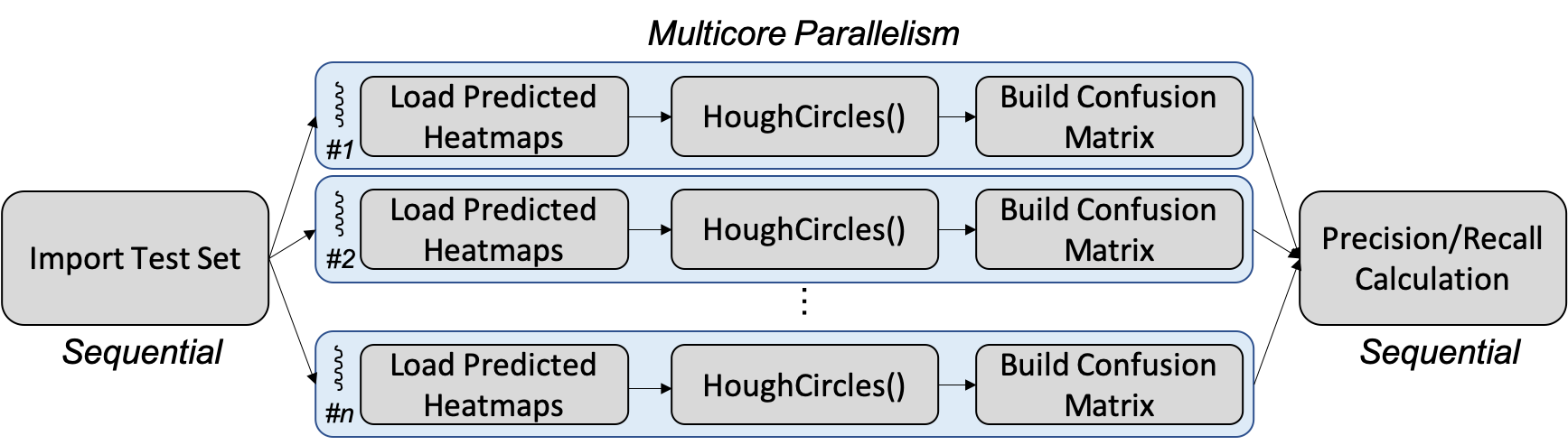
Figure 8: Proposed Parallelism on Task III: TrackNet Model Evaluation.
Experimental Methodology
In this paper, we inspect the real badminton sports video from 2018 Indonesia Open Final - TAI Tzu Ying vs CHEN YuFei. The video is 10 minutes in length and the frame rate is 30 FPS. The resulting overall number of frames is 18,243. The resolution is 1280 by 720.
The entire video is the input of Task I. Task I retrieves all 18,243 frames from the video and saves as jpg files. In a sequential operation, the processing time is 544.16 seconds. Note that the majority of the execution time of Task I lies in saving frames, which is fully parallelizable.
The input of Task II is the label file which specifies the badminton coordinate of each frame. Since the video contains 18,243 frames, Task II is responsible for generating 18,243 heatmaps. The label file is labeled manually using the developed labeling tool. Each row of the label file specifies current frame number, badminton's x coordinate, and badminton's y coordinate.
In deep learning model training, we usually divide the dataset into 70% training set and 30% test set. The purpose of the training set is to train the neural network and the purpose of the test set is to evaluate the model accuracy. In this paper, we follow the 70/30 principle and the resulting test set and training set have 12,771 and 5,472 frames, respectively. Since Task III is to evaluate the trained TrackNet model, the input dataset contains 5,472 images. Those 5,472 test images are fed to TrackNet which generates corresponding predicted heatmaps. Task III collects those predicted heatmaps and exploits the circle detection algorithm, hough circles algorithm, to specify the coordinates of each predicted badminton. The predicted coordinates are compared with the ground truth and categorized into the confusion matrix accordingly based on the error distance with respect to the specification.
The experiments are performed on 2018 MacBook Pro. The CPU is a 6-core 2.6 GHz Intel i7 processor and the system memory is 32 GB with 2400 MHz DDR4. All tasks will be evaluated by one to six cores so that the trend of execution time, speedup, efficiency, and scalability can be thoroughly analyzed.
Experimental Results
In this section, experimental results of Task I, Task II, and Task III are elaborated. First of all, the execution time comparison of different numbers of cores is shown. Then, the speedup and efficiency of parallelism are explained and discussed. At last, the conclusion for each task will be provided.
For Task I, the experimental results of execution time are shown as Figure 9. The execution time of 1, 2, 3, 4, 5, and 6 cores are 544.16, 308.30, 247.09, 221.00, 206.99, and 199.57 seconds, respectively. In the single-core processing, nearly 9 minutes are required to retrieve 18,243 frames from the 10 minutes video. When applying parallel programming, multicore processing can successfully achieve execution time reduction. It can be calculated that at most 344.59 seconds are saved by executing the program with 6 cores. In other words, when exploiting parallel programming and multicore processing, around 5 and a half minutes are saved to retrieve 18,243 frames from a 10 minutes video. The speedup of execution time is quite obvious.
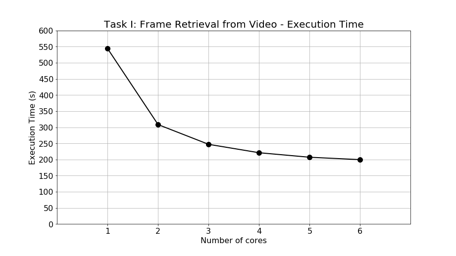
Figure 9: Execution time of Task I: Frame retrieval from video.
Furthermore, the speedup is calculated and shown as Figure 10. The speedup of 2, 3, 4, 5, and 6 cores are 1.77, 2.20, 2.46, 2.63, and 2.73 times faster than single-core processing, respectively. From the figure, it can be observed that the speedup is less as the number of cores increases. This phenomenon is caused by an increasing proportion of the sequential part of the program which is retrieving frames from video when the number of cores increases. Since the sequential program is not parallelizable, the execution time is static regardless of how many cores are executing the task. Once the sequential proportion increases, the speedup starts to deteriorate as expected. As discussed in the programming profiling in previous section, the non-parallelizable part accounts for 11.95% of all program in the single-core operation and such a proportion is not low at all so that the speedup performance is limited.
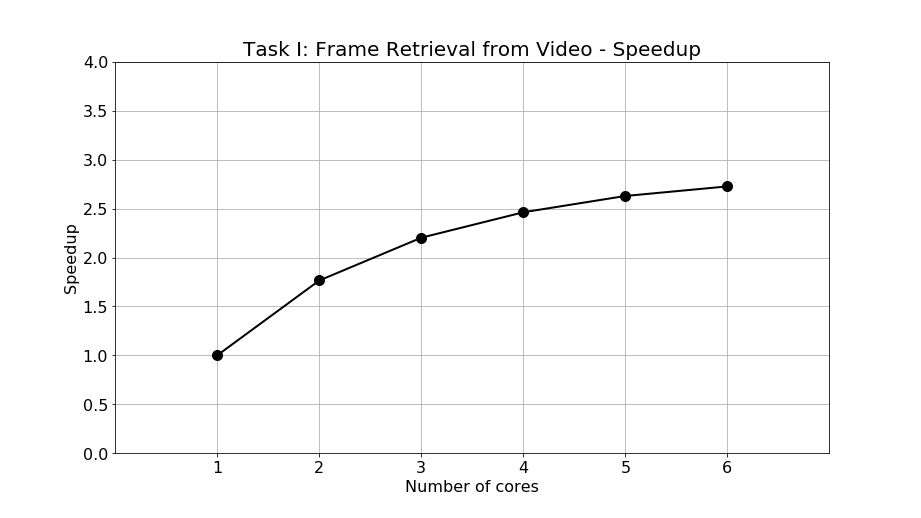
Figure 10: Speedup of Task I: Frame retrieval from video.
Although the speedup deteriorates fast as the number of cores increase, suggesting moderate scalability, the overall time saved is still significant. The moderate scalability is caused mainly by a large proportion of non-parallelizable program which is inevitable. In conclusion, when retrieving and saving all frames from a 10 minutes video, we saved 5 and a half minutes by achieving 2.73 speedup in 6-core multiprocessing.
For Task II, the experimental results of execution time are shown as Figure 11. The execution time of 1, 2, 3, 4, 5, and 6 cores are 2977.31, 1606.48, 1184.15, 953.97, 831.29, and 750.22 seconds, respectively. In the single-core processing, nearly 50 minutes are required to generate 18,243 heatmaps. Compared to Task I, the execution time of Task II is much longer so that the necessity for program acceleration is more desperate. When applying parallel programming, multicore processing can successfully achieve execution time reduction. It can be calculated that at most 2227.09 seconds are saved by executing the program with 6 cores. In other words, when exploiting parallel programming and multicore processing, around 37 minutes are saved to generate 18,243 heatmaps. The execution time reduction is extremely significant, suggesting that the program parallelism has an extraordinary performance.
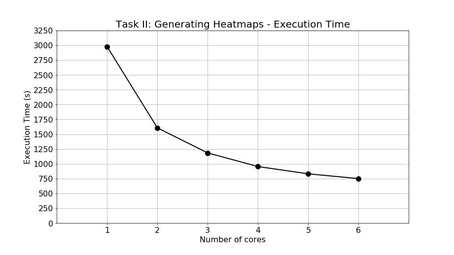
Figure 11: Execution time of Task II: Generating heatmaps.
The speedup is calculated and shown in Figure 12. The speedup of 2, 3, 4, 5, and 6 cores are 1.85, 2.51, 3.12, 3.58, and 3.97 times faster than single-core processing, respectively. The speedup performance is exceptional due to the highly parallelizable characteristics of Task II. As mentioned in previous section, the program profiling of Task II shows that larger than 99.9% of the program are parallelizable. Hence, as the number of cores increases, the non-parallelizable part of the program is still insignificant compared with the parallelizable part, resulting in a large speedup performance when adopting parallel programming. In addition, the entire process of task II does not require data sharing among different processors, so there is no communication overhead in parallel programming.
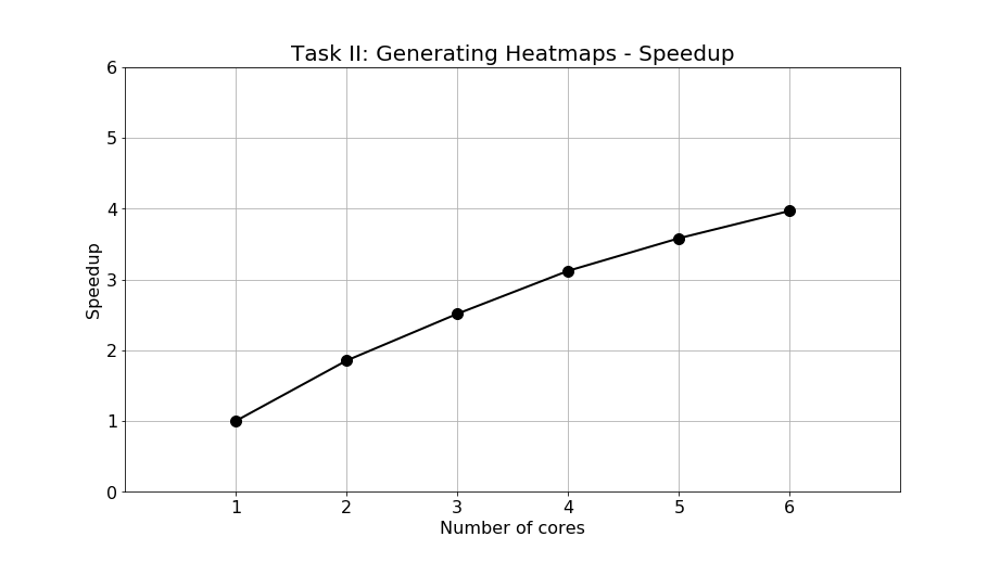
Figure 12: Speedup of Task II: Generating heatmaps.
The exceptional speedup of Task II when adopting parallel programming is extremely beneficial. Without speedup, the user has to wait for 50 minutes to generate 18,243 heatmaps, each has a resolution of 1280 by 720. When turning on the option of multicore processing, only 13 minutes are required to complete the job, saving an immense amount of time. Owing to the highly parallelizable profile of the program, such high speedup can be achieved to save the execution time.
For Task III, the experimental results of execution time are shown as Figure 13. The execution time of 1, 2, 3, 4, 5, and 6 cores are 54.07, 38.84, 36.85, 37.21, 37.39, and 37.85 seconds, respectively. The execution time stops decreasing when the number of cores is larger than 3. After 3 cores, more cores results in a worse performance. The abnormal phenomenon completely exceeds our expectation. The maximum saved time is 17.22 seconds when operating with 3 cores. The performance is poor and the reason causing such problem will be elaborated later.
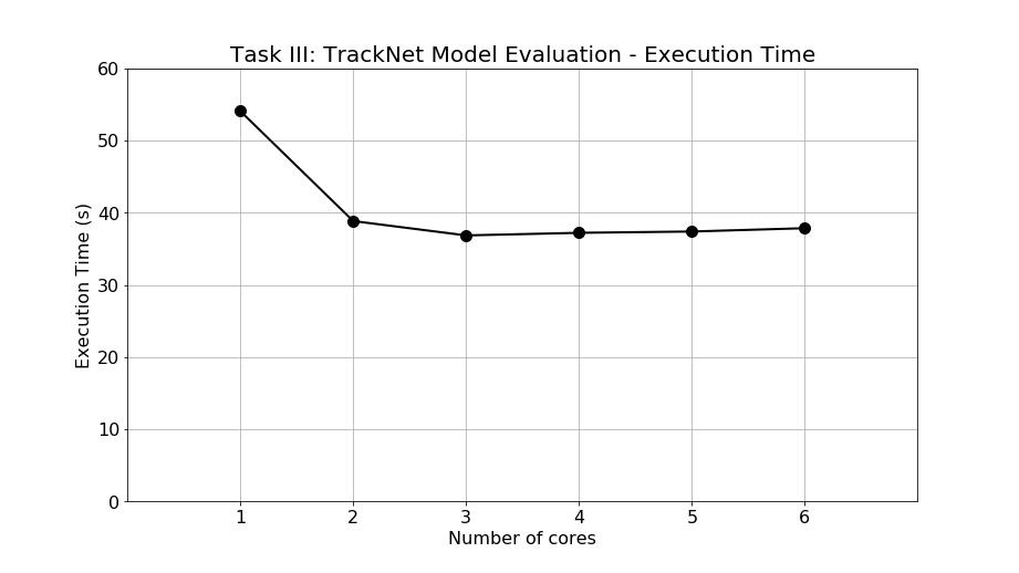
Figure 13: Execution time of Task III: TrackNet model evaluation.
The speedup is calculated and shown in Figure 14. The speedup of 2, 3, 4, 5, and 6 cores are 13.9, 1.47, 1.45, 1.45, and 1.43 times faster than single-core processing, respectively. The speedup stops growing and even start dropping when the number of cores is more than 3. The program profiling of Task III shows that 99% of the program are parallelizable so that the expected speedup should be significant. However, the experimental result is completely opposite to our expectation.
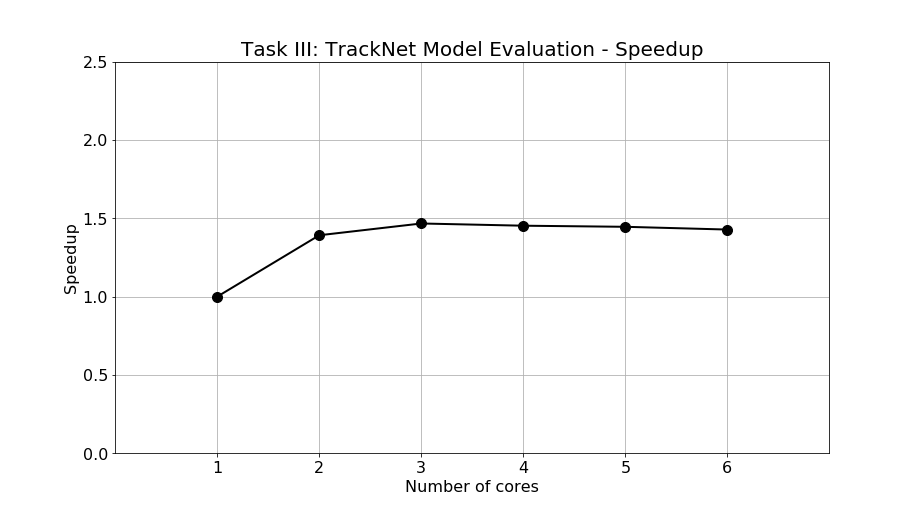
Figure 14: Speedup of Task III: TrackNet model evaluation.
To delve deeper and dig out the root cause of why our parallelism performance is poor, a detailed program profiling against the parallelizable blocks is adopted, including loading predicted heatmaps, detecting circles using Hough Circles function, and building confusion matrix. The profiling is adopted to investigate each blocks' execution time in each iteration and observe the variation of execution time when the number of cores increases. Figure 15 shows profiling result in the single-core execution scenario. Loading predicted heatmaps, detecting circles by Hough Circle function, and building confusion matrix account for 1.682, 8.100, and 0.017 ms, respectively. Namely, loading predicted heatmaps accounts for 17.17%, detecting circles by Hough Circle function accounts for 82.66%, and building confusion matrix accounts for 0.17%. From the profiling, we have found that Hough Circle function dominates the parallelizable program.
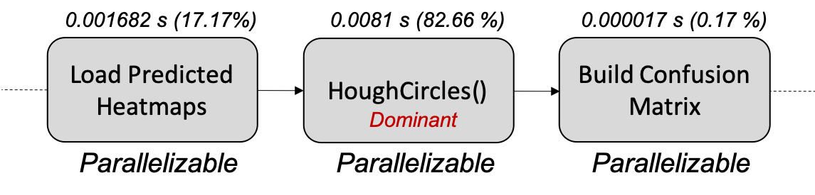
Figure 15: Profiling against parallelizable function blocks of Task III.
Furthermore, we apply profiling when the number of cores increases and the result is shown in Figure 16. Based on the messages conveyed by the figure, building confusion matrix is ruled off from the suspicion of deteriorating the parallelism performance since the execution time is relatively small compared with the other two functions. Also, loading predicted heatmaps can also be excluded from the suspicion due to a much smaller execution time compared to the Hough Circle algorithm although degradation of execution time can be observed when the number of cores increases. However, the deterioration of the Hough Circle algorithm in terms of execution time is severe as the number of cores increases. The execution time of single iteration of 1, 2, 3, 4, 5, and 6 cores are 8.1, 11.7, 16.9, 22.6, 28.5, and 35.4 ms, respectively. With respect to single-core operation, the deterioration factors are 1.44, 2.09, 2.79, 3.52, and 4.37 for 2, 3, 4, 5, and 6 cores, respectively. Hence, the benefit of an extra core is discounted by the deterioration rate so that the overall parallelism performance does not meet our expectation. The reason for the degradation of Hough Circle algorithm in multicore processing is currently unknown and will be researched in the future to improve the performance of the parallelism of Task III.
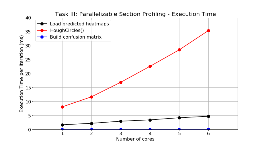
Figure 16: Result of the detailed profiling against parallelizable function blocks of Task III.
Although the performance improvement of Task III is not as significant as Task I and Task II, the benefit brought by parallelizing Task III is momentous. The reason is that Task III is frequently executed when evaluating the performance of the trained TrackNet model. To optimize the parameters of circle detection, the program of Task III has to be modified over and over until a set of optimized parameters is found. With parallelism, the overall execution time of Task III is improved from 54.07 to 36.85 seconds, saving 17.22 seconds of the user's waiting time. The saved time might seem not as much as Task I and Task II, but the actual working efficiency of the user is enormously improved. Future work will be conducted on the further improvement of Task III parallelism by resolving the deterioration effect of Hough Circles algorithm.
Conclusions
Applying parallelism techniques to TrackNet is proved to be beneficial. A significant amount of execution time can be saved for both image pre-processing and post-processing in the TrackNet flow, allowing TrackNet to operate more efficiently than before. Scenarios, proposed solutions, and experiments are all elaborated in this paper. For Task I: Frame Retrieval from Video, 6-core multiprocessing achieves 2.73 speedup and the total saved time is 344.59 seconds. For Task II: Generating Heatmaps, 6-core multiprocessing achieves as high as 3.97 speedup and the total saved time is 2227.09 seconds. For Task III: TrackNet Model Evaluation, 6-core multiprocessing achieves 1.47 speedup and the total saved time is 17.22 seconds. Future works of parallelizing Task III's Hough Circle algorithm will be conducted to further improve the performance of Task III. The source code is available here.